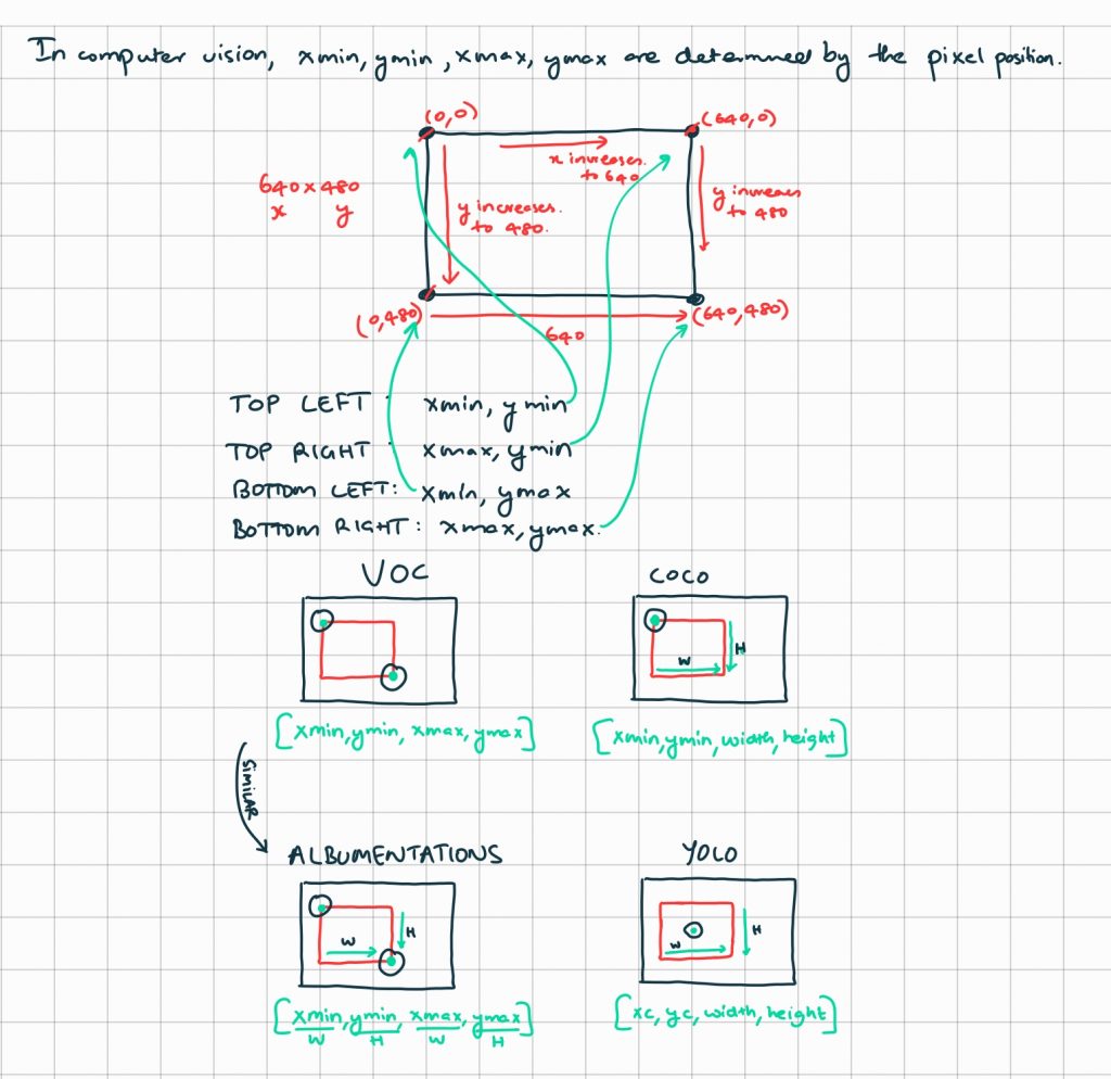
Throughout my whole life, I’ve only heard of and thought in terms of the cartesian coordinates. For images and nD signal processing, as far as I’ve seen, everything is denoted in an “inverted” cartesian coordinate system. It helps to visualize the image array in a row-column indexing format, like in a NumPy array. When I first got introduced to image processing this felt so weird.
For example, in classic 2D image processing, the origin (0, 0) is placed at the top-left corner and the horizontal (n1) axis is the width and the vertical (n2) axis is the height of the image, such that the bottom-right coordinate is (n1, n2). More on that here, a course on image processing that covers the fundamentals of nD spatial and temporal signal processing in detail!
Below is a simple illustration to “illustrate” the various bounding box geometries used in computer vision.